
Journal of Clinical Images and Medical Case Reports
ISSN 2766-7820
Review Article - Open Access, Volume 5
Implant-screw loosening - Part 2: US monitoring proposals
Jacob Halevy-Politch*; Ilan Rusnak
Aerospace Engineering, Technion City, Haifa, Israel
*Corresponding Author : Jacob Halevy-Politc
Aerospace Engineering, Technion City, Haifa, Israel.
Email: yapo@actcom.co.il
Received : Mar 26, 2024
Accepted : Apr 19, 2024
Published : Apr 26, 2024
Archived : www.jcimcr.org
Copyright : © Halevy-Politch J (2024).
Abstract
New US methods for monitoring the loosening/integration in-vivo and intra-operatively are proposed. The first is based on the JetGuide principle, and the others - are based on transmitting the US signal through a conventional implant, or through a new hollow implant that is proposed here. The hollow-screw method is developed further into several versions of measurements: discrete, continuous, circumferential, all using reflected signals, and an interferometric (Mach-Zebder) measuring using one-directional signals.
Citation: Halevy-Politch J, Rusnak I. Implant-screw loosening - Part 2: US monitoring proposals. J Clin Images Med Case Rep. 2024; 5(4): 3014.
Introduction
The methods that already exist for monitoring osseointegration/loosening processes, and quantifying the existing condition of the liquidized gap, between the implant and the bone surrounding it, are described in [1] and are summarized as follows:
Mechanical methods: Apply Pull-Out and Torque (POT) methods and require ISQ (Implant Stability Quotation) for a complete data analysis. These methods are ex-vivo and invasive.
Static non-invasive methods: Using radiography and/or CT, followed by an observation of a halo (on the liquidized gap between the implant and the bone) during measurements from their images. The halo thickness measuring accuracy depends on the person who performs the evaluation; thus, it is a subjective one. Moreover, the patient accumulates over time a high dosage of X-ray radiation and the methods are ex-vivo.
Dynamic methods: Resonance Frequency Analysis (RFA) - where the implant is excited to vibrate by (i) mechanical means (such as mechanical impact), or (ii) Laser excitation while detecting it by laser Doppler reaction/resonance method. These are in-vivo methods, where an interpretation of the obtained results is required.
A different approach was suggested, where a pulsed oscillating source was inserted in the prosthesis and operated remotely; its detected signals are transmitted with acoustic emission signals from the implanted bone. Both signals are collected by an amplifying and processing unit and further analyzed.
The following describes new US methods for monitoring the loosening/integration in-vivo and intra-operative measurements. One of them (The Ultrasonic Flash Light) is based on the existing implant and the JetGuide principle of US monitoring, whereas most of the others are based on transmitting a US signal (pulse, or CW) on a conventional implant, or through a new hollow implant with ‘windows’, as proposed here. This last method was further developed in several monitoring versions containing discrete, continuous, and circumferential (all of them based on the reflected signals); where the interferometric (Mach-Zebder) is based on one-directional signal propagation, with the inherent benefits.
Non-invasive monitoring of loosening, in-vivo and intraoperative
We propose here non-invasive, in-vivo, and intraoperative methods for monitoring the loosening process of an implant inserted in a bone. These methods are based on Ultrasound (US) wave propagation that monitors thickness variations over time, of the thin liquidized layer (>1 mm) between the outer surface of the implant and the cortical bone surrounding it. This thin layer, named in radiography the ‘halo zone’, is defined there by the ‘lucent ring’. When there is an integration process, this thin layer shrinks with time; while loosening occurs - it becomes wider.
It is our interest to follow the progress of these changes and especially their increasing thickness with time (swelling) - causing loosening. These processes are slow and take time; monitoring at equal periods will minimize the measuring ambiguities;
The following describes the proposed solutions as presented in this paper:
The Ultrasonic Flash Light (Ch .4)
Regular implant excited by US (Ch. 5)
A hollow implant with ‘windows’ (Ch. 6)
Integrated gap measurement along the circumference of the implant (7..1)
Angular variation of a US “knife-edge” beam. (Ch. 7,2)
Improved method to monitor loosening, using a hollow implant with ‘windows’ and beam splitters (BS) (Ch. 8)
Continuous measuring solution (Ch. 9.1)
Monitoring loosening along the circumference of the implant (Ch. 9.2)
Interferometric Monitoring of the thin layer by the US (Ch. 10).
These methods are described in more detail in the following chapters.
The ultrasonic flash light
Our previous paper [1] revealed that nowadays there is no Ultrasonic (US) method for the objective measurement of loosening.
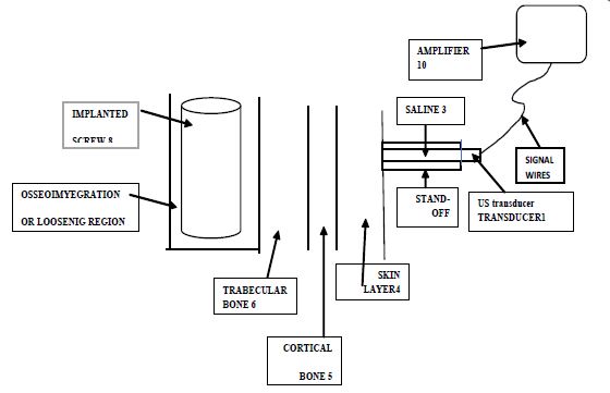
The following proposed monitoring method is based on the principles of “JetGuide” [2-10], where the US wave propagates through a saline (usually of a thin laminar flow) and operates as an A-scope, for measuring the residual distance (or depth) in a drilled bone. This method also enables us to measure changes in depths/distances.
In the case presented here, the US of the measuring system has to pass through a relatively thin layer of cortical bone, usually covered by a soft tissue of skin layer, followed by propagation through a layer of trabecular bone, and after that, it impinges the thin (liquidized layer) and finally, the implant itself - thus, measuring the width of the loosening layer. This is schematically presented in Figure 1.
The stand-off tube is required so that only the ‘far field’ of the US will enter the inspected tissue. Our interest is to measure the distance between the boundaries denoted 5 and 6 in Figure 1, which is the width of the loosening layer. Figure 2 presents a hypothetical reflection pattern. Therefore, we propose to apply a US beam that will propagate through the mentioned layers and monitor the width changes of the loosening layer.
An important issue in this monitoring method is the selection of the US frequency. A preliminary frequency selection procedure is outlined in Appendix A.
Transmission through the cortical bone requires lowering the frequency, as the attenuation decreases with frequency lowering. On the other hand, the thin loosening layer requires high resolution - thus, a high frequency is essential. This issue requires thorough treatment that involves a trade-off, including measurements of the in-vivo mechanical properties of the loosening material, of the cortical bone the trabecular bone, and of the implant (such as SOS, impedance, specific density, Young’s modulus, reflection coefficients) and thorough analysis, optimization, and in vivo measurements. Also, it requires knowledge of the measured noise level and its spectrum.
Other issues include such as the required transmitter power, the transmitted waveform, signal processing, type of amplifier, low noise amplifiers, the dynamic range of the amplifiers, availability of transducer, and safety considerations.
Special care must be given to minimize the amplitude of the US wave, its duration, and the total energy applied during the measurement process as excessive amplitude, duration, and energy can harm the already existing osseointegration.
The design process and product development should be accompanied by suitable measurements in vivo and at different locations of the human body.
As mentioned, this paper highlights new directions for monitoring loosening, by using US methods, where this is one of the proposals. Since it is based on previous knowledge of similar measurements, it looks like its potential is promised for realization.

Regular implant excited by US
Transmitting a US signal, with high enough energy, that impinges on a regular implant, inserted in bone, will cause its resonant vibration. The reflected signals from the incident surface by the transmitted one, are detected and represent the implant’s response.
The implant is modeled here by a metallic cylinder, as described in Figure 3.
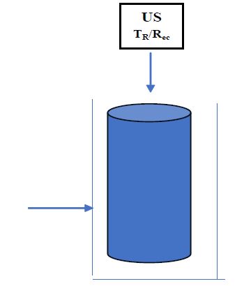
US-transmitted waves are incident vertically to the implant, on its upper circular surface. The US signal is transmitted and received through a thin jet of saline - as described already in the JetGuide methods for monitoring the US reflected signals [2-10]. The outlet, through which the thin saline stream flows (and through which the US wave propagates in both directions), is placed close to the upper side of the implant.
Assuming, d [mm] is the width of the thin liquidized layer, created during implantation, between the implant and the bone tissue surrounding it. A resolution of (d/10 to d/20) is required to monitor changes that occur over time. Therefore, for a US monitoring system, using a train of pulses that will be able to resolve these changes; or by applying a Modulated Continuous Wave (MCW) that measures the phase between the reference (transmitted) and the reflected signals. For example, using a modulation frequency fm = 30 kHz, at a velocity of 1.5 x 10³ [m/sec], the wavelength λ[m] = c f-1 = 5 x 10⁻² [m] = 50 [mm]. If λ = φ, which can be divided into 400 parts, it provides a possibility to follow incremental changes over time of 0.125 [mm], which satisfies the conditions for the ‘follow-up’ on loosening.
According to the ‘Time of Arrival’ of the echoes, this method may resolve between those arriving from the bottom part of the implant and its sides at several heights; However, this method will not be able to differentiate between directions at the same height.
Another possibility is to transmit high-energy US pulses (within the limits permitted by FDA, in order not to overheat the surrounding tissue), which will cause to implant of a resonant vibration - as described in [1] for the pulsed laser method. The resonance amplitude is affected by the loosening/osseointegration conditions. However, when loosening occurs, the resonance peak almost disappears, which was found experimentally by simulation [1].
A hollow implant with ‘windows’
General requirements: The US signal is transmitted and received in a similar way as in the method described in the previous chapter. Figure 4 presents schematically the proposed hollow implant with windows in its surroundings.
According to the described in Figure 4, this kind of implant can discriminate between several heights and directions (conditionally that window’s direction is known). The drawback here is that it provides discrete angular information, whereas a continuous one will be preferable.
Requirements for the improved implant:
US Beam Splitter (BS) in front of every hole/window in the implant’s wall;
The US BS should have the ability of US propagation in both directions;
The whole implant should be filled with saline and be sealed hermetically apriori;
The US is capable of propagating in both directions through the ‘window and membrane (made from a suitable elastic material). The first ‘window/membrane’ is placed at the implant’s entrance (between the outlet of saline flow and the implant); the others - are at the circumference of the implant’s wall;
Leakage should be completely prevented;
Signal processing has to discriminate between reflected signals from different windows (thus providing height information). This will enable monitoring of small thickness changes of the thin liquidized layer (>1 mm);
Applying a swept signal, such that its intensity increases with time, might solve the height/depth resolution (i.e., less intensity for closer window/s to the entrance of the signal and higher - to deeper/further one).
The direction will be solved, if there exists a possibility to obtain a US wave in the shape of a “rotating knife edge”. In this case, it will be possible to rotate the beam and define the direction of the monitored window in the implant.
Implant’s bottom: It is assumed, that while considering the bottom part of an implant, there exists also a gap (thin layer) of d > 1 mm, between its outer surface and the cortical bone tissue surrounding it (that was drilled for inserting the implant). The material in that gap is known [1] because of its liquidized nature, with a US velocity of about 1.5 x 10³ m/sec (similar to that of water); It is expected that this thin layer will shrink with time and its material will transform to a crystalized solid, close to the properties of a cortical bone - named osseointegration. However, if the opposite occurs, and it is a widening process of the loosening process occurs the liquidized layer will be in a higher volume.
To follow this process (shrinking or swelling), a monitoring method is proposed here, using short US pulses, or modulated continuous US waves - MCW). The transmitted signals propagate through the implant and their echoes are obtained from both interfaces of this thin layer - thus enabling us to measure the ‘time difference’ of their arrivals. Since the velocity of propagation is known, the thickness of the layer can be calculated [4,6]. It should also be considered that this measurement is performed in the US near field (NF) - as described in more detail in Appendix B. Thus, as the thickness increases, the reflected signal is smaller which reduces the detectivity - causing ambiguities in its interpretation.
Monitoring the circumferential gap thickness of the Implant: The main requirements of the system:
Measuring the thickness of the gap between and along the circumference of the implant and the cortical bone.
Angular orientation variation of a US “knife beam”.
US thickness measurement of the thin layer, at discrete points.
Low-frequency Continuous Wave (CW) US in a ’transmission mode’ and monitoring the phase difference (with high accuracy) between the transmitted and reflected signals.
Integrated gap measurement along the circumference of the implant
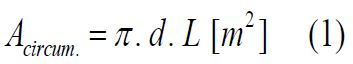
An implant of diameter d [m] and length L [m] is assumed. Its circumferential area is:
Near Field (NF) length is according to eq. (B.5).
Accordingly, if we assume an implant of diameter d=3 mm, with a length L=3 cm, a monitoring US frequency f=10 MHz = 107 Hz, and a velocity of US propagation in the gap region c = 1500 m/sec, one obtains a NF length of N=45 mm.
Accordingly, measuring a gap with a thickness between 1 to 2 mm belongs to the beginning of the near field zone, where the attenuation is high [12], of the order of 5 dB in each direction, at f=10 MHz.
Assuming an input of US pressure I1, due to the acoustic impedance Z1 at the entrance to the thin layer (gap), a reflection occurs and the transmitted pressure amplitude is according to [4,6]:
To find out the value of the reflected signal, this calculation
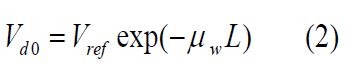
can be followed after the references already mentioned in [4,6].
Angular variation of a US “knife-edge” beam
(using a relatively thin aperture with a lens system, suitable for the US bandwidth).
A ‘knife edge’ beam configuration: Let us assume that a circularly shaped US bean is incident a thin rectangular aperture. Thus, behind this aperture, one obtains a ‘knife edge’ beam. While rotating this aperture, a rotatable ‘knife edge’ beam rotates as well; both are rotating in synchronization. Assuming that the angular position of the slit (the narrow rectangle) is known at every moment, causing the direction of the transmitted ‘knife-edge’ US beam, is also known - thus it provides the required ‘angular information’.
How is the US beam transmitted and received through the implant?
The US Beam-Splitter (BS) is described schematically in Figure 5.
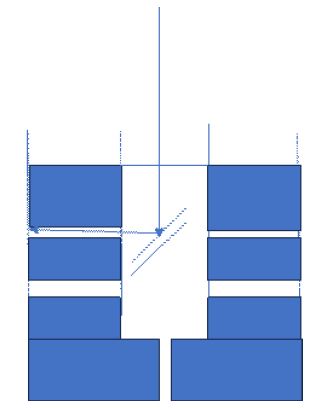
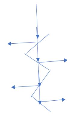
It is assumed that the US beam propagates along the main (symmetric) axis of the hollow implant. To tilt (change the direction of propagation) part of this beam, a BS is inserted at that location; it directs part of the incident beam at 90 deg. toward the circumferential area of the implant (the thin layer with liquidized material); the rest of the US beam continuous to propagate through the BS, toward the lower part of the hollow implant, where is performed a similar beam-tilting for measuring the thickness of the thin layer, but at a different height. This method of tilting the US beam is repeated several times.
The US ‘window': The ‘window’ is the element in the hollow implant, through which the US beam is transmitted toward the thin layer, and reflections from this layer are received back (on the same US transducer), processed, and displayed. The main properties of such a ‘window’ are:
It has to be completely sealed in both directions.
To enable transmission of US intensity in both directions (with a negligible attenuation) and no distortions of the front surface of the US beam are assumed.
Elastic thin membranes were already applied for similar purposes [13].
The US Windows - conclusions: It is assumed that all the windows in the hollow implant are in the range of [1 to 1.5] mm in diameter. Conditions for an elastic window: if the reflections of the US pressure intensity are in the range of [(-10) to (-12)] dB (relative to the incident intensity), the transfer of beam intensity will be without distortion and further attenuation.
Assuming these small apertures, of (1 to 1.5) dia mm, only the direct reflections are considered (perpendicular to the window).
In summary: due to the small window’s aperture and the relatively long and narrow path along the hollow implant, only axial reflections will arrive at the detecting US transducer’s surface.
Improved method to monitor loosening, using a hollow implant with ‘windows’ and Beam Splitters (BS)
Required properties
The implant is hermetically sealed.
It is filled with saline solution.
The windows are transmitting and receiving the US waves without distorting them.
(iv) These windows are made of a thin layer of elastic material.
It is assumed that the hollow implant diameter is between 3 to 4 mm; therefore, the window’s diameter is between 1 - 2 mm. Accordingly, all the windows in this type of implant, are ~ 1.5 mm in diameter.
In this small volume of the hollow implant, the BS is in a constant position. These BSs are described schematically in Figure 5:
A continuous measurement: Proposed here is a hollow implant, made from a transparent material to US waves that will enable a continuous measurement of the thin layer. We apply here the same measuring method, as it was presented above; however, there is a possibility to perform a continuous measurement, at every angular position.
These kinds of implants are molded, causing to much smaller production cost than for a similar metallic one, especially if it is a hollow one and contains the ‘windows’ mentioned above.
Monitoring loosening along the circumference of the implant
The general layout: We present here two methods for monitoring loosening along the circumference of the implant.
The solution presented in the previous section provides loosening information in a discrete direction of a window and the BS - located in the implant.
Components of the new method:
Instead of applying a circular US beam, it is modified to the shape of a thin rectangle.
The slit rotates in synchronization with the BSs.
Instead of discrete windows, there are imposed “circular (ring) windows” that enable monitoring of the loosening thin layer circumferentially, in 360 deg.
Thus, the direction at every monitoring sequence is obtained from the directional position of the thin-shaped rectangular beam.
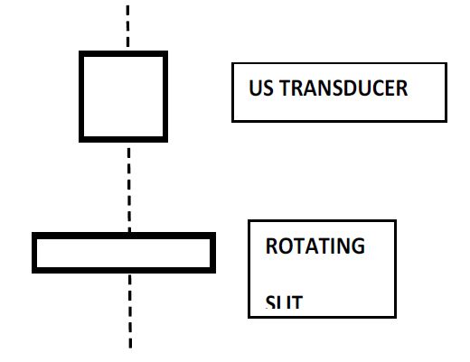
Methods for obtaining the slit: Figure 6 describes the simplest case, where at a distance larger (at least twice) than the Near Field (see Appendix B), a slit is placed. However, intensity losses are obtained in such a simple scheme.
To overcome the drawback of the mentioned intensity losses, it is also possible to apply a set of suitable US lenses (similarly as it is done in optics) that will concentrate the US wave, thus causing a relatively negligible intensity loss, followed, as before, by a rotating slit, as described in Figure 7.
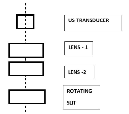
The method described in Figure 7, enables us to identify the loosening circumferentially, where the rotations of the BS and the slit are synchronized.
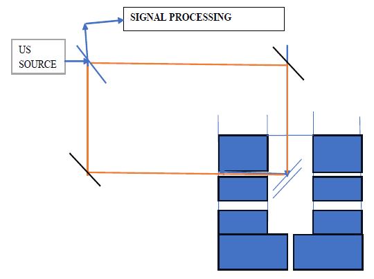
Interferometric Monitoring of the thin layer by the US
Measuring principle: Presented is a Mach-Zender interferometric method [13,14], using US waves, at a frequency of 300 kHz, for monitoring changes of the thin layer. The principal system is described schematically in Figure 8. This method monitors thickness variations with high accuracy, and also their direction - widening or shrinking. In this method, the US waves propagate only in one direction through the thin liquidized layer (and similarly in other tissue layers); thus, the attenuation is about half of that in a reflecting system and the required US power is also smaller than in a reflecting method.
This monitoring method is based on phase difference measurement Δφ, between a ‘direct’ (reference, or unperturbed) beam and the other beam that contains information of interest (in this case, about the thickness of the thin layer). Here φ [deg] is the phase of the US wave λ [m]. The phase φ can be electronically subdivided into 400 or 1000. Therefore, for
λ|3 105, c=1.5 103 = 5 10-3 m / λ = 5 mm
Therefore, (λ/100) = 5 10-5 m = 50 μm (that satisfies the requirements of following thickness changes).
Notes
1. For monitoring in different directions and heights, one should change the position of the Mach-Zemder Interferometer (MZI).
2. Using a solid-state micro-Mach-Zender interferometer, it is possible to perform all these measurements simultaneously.
Calibration, repositioning, and safety in long-term measurements
Calibration
While loosening is considered, it may be a process that has to be followed over several years [1]. In these cases, one has to be aware that all the measuring conditions are the same throughout all that time. This requires, before every measurement is performed, re-calibrating the measuring system [17,18]. This is performed against a standard device or a system. The environmental conditions should also be the same in all measurements. All these data should be enrolled in the protocol.
Repositioning
For the same reasons as for recalibration, the importance of ‘repositioning the “measuring device” was found of the same importance. For these purposes, every type of implantation has its specific location [19-20]. Moreover, there may be cases that will require a repositioning device for the same part of the body, but at different placement (or different anatomical shape or size). There should be overviewed cases, where a repositioning device will be able to serve (be adapted) a larger population.
The accuracy of a repositioning has to be higher than the required monitoring resolution, without causing an ambiguity in the obtained data.
Safety
This section reviews shortly the maximum US intensity permitted on human tissue (according to the FDA).
The following values values are defined as:
Ipi: pulse-intensity integral.
Ipi.3: attenuated pulse-intensity integral.
Ita: temporal-average intensity.
Isata: spatial-average, temporal-average intensity.
Ispta: spatial-peak temporal-average intensity.
Ispta.3: attenuated spatial-peak temporal-average intensity.
K: thermal conductivity.
MI: mechanical index.
TI: thermal index.
The intensity incident on an area (surface) is limited according to:
Derated ISPTA≤720 mW/cm2,
and either MI≤1.9, or Derated ISPPA≤190 W/cm2.
These intensity values should be taken into consideration while considering the development of the proposed US monitoring of loosening while it impinges on human tissue.
Summary
The existing monitoring methods for loosening have some drawbacks, as some of them are ex-vivo, and are dependent on the operator, the data analyzer, and its interpretation; whereas others apply X-ray that is accumulated over time to high dosage.
As a consequence, we proposed here nine in-vivo and intraoperative methods, based on US waves. The first one applies the principles of JetGuide monitoring that emits and receives the US pulsed signals through a thin pipe filled with saline. The other eight methods (except one) are based on a new hollow implant, with windows (or US transparent rings) in its circumference. All these methods are planned to operate in the lower range of the US, due to the required propagation through the Near Field, located close to the zone of measurement (in the thin layer, between the implant and the cortical bone tissue) and also (mainly) through the cortical layer of a bone.
To achieve measuring accuracy over time, attention should be paid to the required recalibration of the system before every measurement, as well as to the repositioning device that will bring the measuring system to the same position of measurement, with an accuracy better, or at least the same, of the measured one.
References
- J Halevy-Politch, I Rusnak, Implant screw loosening. Part 1: Review of the existing methods.
- N Rosenberg, A Craft, J Halevy-Politch. Intraosseous monitoring and guiding by ultrasound: A feasibility study, Ultrasonics. 2014; 54: 710-714.
- N Rosenberg, J Halevy-Politch. Intraosseous monitoring of drilling in lumbar vertebrae by ultrasound: An experimental feasibility study, Plos One. 2017. https://doi.org/10.137/1/journal.pne.0174545.
- I Rusnak, N Rosenberg, J Halevy-Politch. Trabecular bone attenuation and velocity assess by ultrasound pulse echoes, Applied Acoustics. 2020; 157: 107007. https://doi.org/10.1016/j.apacous.2019.1007007
- J Halevy-Politch, M Zaaroor, A Sinai, M. Constantinescu, New US Device versus imaging US to assess tumor-in-brain, Chinese Neurosurgical Journal. 2020; 6(28). https://doi.org/10.1186/s41016-020-00205-1.
- J Halevy-Politch, I Rusnak, N Rosenberg. Novel intraoperative US ץmethod to assess the SOS in trabecular bone, Baltica. 2017; 33(7). ISSN:0067-3064.
- M Zaaroor, G Sviri, A Sinai M. Constantinescu, and J. Halevy-Politch, Intraoperative spinal cord remote monitoring with a modified US A- scope, Austinpublishinggroup.com/clinical-case-reports/fulltext/ajccr-v8-id1219. php# Top. https://doi.org/10.26420/austinjclincaserep.2021.1219
- J Halevy-Politch, A Craft, N Rosenberg. US Patent. 2010; 7(748): 273-B2.
- E E Machtei, H Zigdon, L Levin, M Peled. Novel Ultrasonic Device to Measure the Distance from the Bottom of the Osteotome to Various Anatomic Landmarks, J. Periodontol, July. 2010; 1051-1044. Doi:10.1902/jp.201009021.
- H Zigdon-Giladi, M Saminsky, R Elimelech, E E Machtei. Intraoperative measurement of the distance from the bottom of the osteotomy to the mandibular canal using a novel ultrasonic device. and guided by ultrasound: A feasibility study”, Clinical Implant Dentistry and Related Res. 2015; 18(5): 1034-1041. https://doi.org/10.1111/cid.12362
- S. Mensah and E. Franceschini, Near-field ultrasound tomography, J. Acoust. Soc. Am. 2007; 121: 1423-1433. https://doi.org/10.1121/1.2436637
- Gao W, et al. Study of Ultrasonic Near-Field Region in Ultrasonic Liquid-Level Monitoring System. Micromechanics. 2020; 11: 763. doi:10.3390/mi11080763.
- KP Zetie1, SF Adams, RM Tocknell. How does a Mach-Zehnder interferometer work?. Phys. Educ. 2000; 35(1): 35-46 https://doi.org/10.1088/0031-9120/35/1/308.
- Fundamentals of Optical Waveguides (2nd ed.). Access through Univ. of Toronto, Science Direct. 2006; 417-534.
- F Mandelkorn, N H Farhat. Progress Report on The Application of m-Wave Imaging, applying US detecting methods. The Moore School of EE, U of Pa. 1973.
- C Zhou, Y Wang, C Qiao, W Dai. Calibration Method of an Ultrasonic System for Temperature Measurement, PLOS ONE. 2016. https://doi.org/10.1371/journal.pone.0165335
- L R Zdero, P Fenton, JT Bryant. A digital image analysis method for diagnostic ultrasound calibration. Ultrasonics. 2002; 39(10): 695-702. https://doi.org/10.1016/S0041-624X(02)00383-9.
- S U Butt, JF Antoine, P Martin. An analytical model for repositioning of 6 D.O.F. fixturing system, Mech. And Ind. 2012; 13: 203-217.
- Z Zhu, C Zhao. Angular error measurement of a workpiece. repositioning using a full-scale rotation detection method, Optics Express. 2023; 31(3): 4813. https://doi.org/10.1364/OE.481137.
- Walsh Conor J, Slocum Alexander H, Gupta Rajiv. Preliminary. evaluation of robotic needle distal tip repositioning. URI: http://hdl.handle.net/1721.1/79090. Massachusetts Institute of Technology. Department of Mechanical. Engineering, Proceedings of SPIE; v. 7901.
Appendix A: Preliminary frequency procedure selection
Frequency selection
The following is a preliminary frequency selection procedure.
An artifact (defined as a region of spherical shape with a different reflection property) located at distance R in an attenuating media, which is homogeneous along the US propagation path, is measured. The problem is to select the transmitting frequency, to achieve minimal error during a measurement.
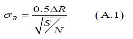
The measurement accuracy is defined as
Where:
ΔR is the required resolution [m]
S/N is the obtained signal-to-noise ratio (SNR).
The resolution is:

Where:
c is the speed of sound in the media; in our case, c = 1500 [m/s]
τ is the duration of the rectangular transmitted pulse [s].
The transmitted rectangular pulse is composed of n sinewave cycles of frequency f [Hz].
That is:
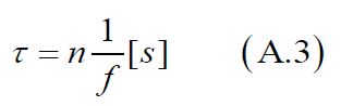
Where:
f is the frequency [Hz]
p = 1/f is the duration of one cycle [s]
n is the number of cycles in the rectangular pulse.
Finally,
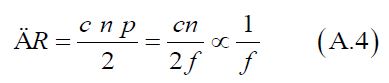
The optimum of ΔR depends on the different media along the path of measurement with frequency.
The SNR is as follows:
The received power, P_r is given by (from an artifact along the measured path)
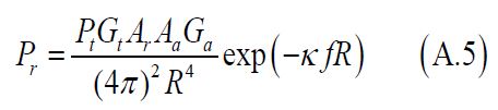
At is the area of the transmitting (Tr) transducer [m2]
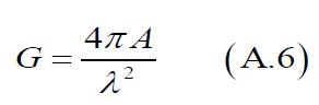
λ is the wavelength [m]
λf=c (A.7)
Ar is the area of the receiving (Rec) transducer [m2]
In the case that the single transducer is used, i.e. Tr = Rec, then At = Ar.
Aa is the area of the artifact [m2]
Ga is the gain of the artifact
σa is the US cross-section of the artifact,
σa=Aa Ga (A.8)
It is assumed that σa is frequency independent
Gt is the transmitted radiation pattern
Gr is the receiver pattern
In the case that the same transducer is used for transmitting and receiving, Gt = Gr.
κ is the slope of the attenuation [1/Hz/m]
R is the measured range [m]
Accordingly, we have

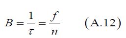
The noise power is
N=kT0 BNF ̅ [W] (A.10)
B is the bandwidth of the signal processing [Hz]
k is the Boltzmann constant = 1.38×10⁻²³ [joule/K]
T0 is the ambient temperature. T0 = 290 [K]
NF ̅ is the noise figure of the preamplifier
Further, for matched filter
Bτ=1 (A.11)
Therefore
and
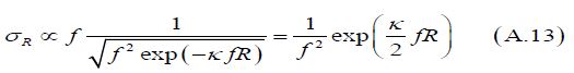
A.2 Frequency Optimization
For the minimization of measurement error, we have
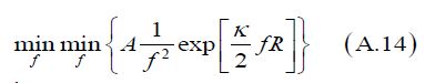
To find the minimum, we require
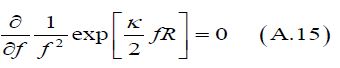
and after the derivation:
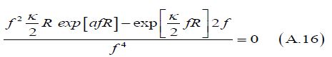
From where it follows
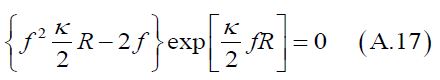
Thus, the “optimal” frequency is:
The optimal frequency for minimizing the measuring error is inversely proportional to the distance R, where the artifact distance is measured. As the distance increases the frequency should be lowered.
The length of the stand-off tube
The stand-off tube was described in “The Ultrasonic Flash Light”.
The stand-off length should be as long as the length of the near field zone and greater than the ‘blind range’ (defined in the following paragraph). The near field zone at 50 MHz is
The length of the stand-off tube is large, so the frequency must be lower than 50MHz.
(This coincides with the requirement of using lower frequency, mainly due to the attenuation in the cortical bone).
The blind range
The blind range is
The parameters of (A.20) were defined in previous sections.
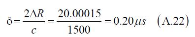
It would be constructive that the stand-off tube length be matched to the blind range. At 300KHz the blind range is:
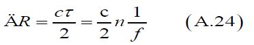
The required resolution
Assuming that the required resolution is 0.15mm
Then
As pf=1
where p is the duration of one transmitted pulse [s]
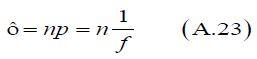
this means that the accuracy increases with frequency.
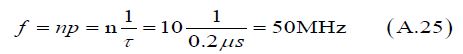
For sufficient energy assume there are 10 pulses/ burst the frequency that is obtained
Interferometric measurement
By assuming that there are two artifacts, then the received signal will be
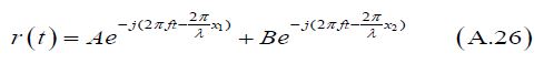
We have one measurement and need to obtain two unknowns, x1 and x2.
By measuring at two frequencies, the two unknowns are derivable.
Generally, this requires a wide bandwidth signal, like a spread spectrum waveform, chirp waveform, or a High-Range Resolution (HRR) waveform. Wideband waveform requires transmitting in a very large bandwidth, like 5MHz, to obtain a resolution of 0.2μs.
Table A1: Summary of parameters playing a role in the measuring system.
| No. | Resolution ΔR | Accuracy S/N=20dB | Pulse length τ | Cycles per pulse n | One cycle period p | Frequency f | wavelength | Far-field - N | Blind range Rb |
|---|---|---|---|---|---|---|---|---|---|
| [mm] |  @ S/N=20dB [□m] @ S/N=20dB [□m] |
 [‘□sec] [‘□sec] |
p=1/f p=1/n [□sec] |
f=1/p [kHz] | λ=c/f [□m] |
 L=3m [cm] L=3m [cm] |
[mm] | ||
| 1 | 0.15 | 7.5 | 0.2 | 10 | 0.02 | 50 103 | 30 | 15 | 0.15 |
| 2 | 0.15 | 7.5 | 0.2 | 5 | 0.04 | 25 103 | 60 | 7.5 | 0.15 |
| 3 | 0.3 | 15 | 0.4 | 5 | 0.08 | 12.5 103 | 120 | 3.75 | 0.3 |
| 4 | 0.3 | 15 | 0.4 | 2 | 0.2 | 5 103 | 300 | 1.5 | 0.3 |
| 5 | 7.5 | 375 | 10 | 3 | 3.3 | 300 | 5 103 | 0.9 | 7.5 |
| 6 | 24.75 | 1200 | 33 | 10 | 3.3 | 300 | 5 103 | 0.9 | 24.75 |
Table 1 summarizes the parameters (such as frequencies, resolution, pulse length) that play a role in a measuring system.
Appendix B
The ‘Near Field’ problem
The ‘near field’ - definition
In all the cases mentioned in the paper, the US measurements are performed in the ‘near field’ [11, 12], as described graphically by Gao [12], where there are described near and far field regions along a propagation path of the US wave.
The near field region N is defined as:
Performing a calculation for f = 300 kHz, one can find that N = 45 mm, which means a 3-times longer region of the near field, i.e. requiring
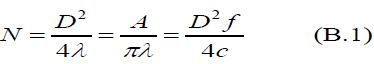
where
D is the US transducer active diameter [mm]
A is the US transducer active area m[m2]
□ is the US wavelength [mm]
And
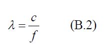
where
c is the US wave velocity in the medium [m/sec]
f is the US frequency [Hz]
In the case discussed here
D=3 mm
f=10 MHz
c=1500 m/sec
Thus

Improved detecting resolution: If the gap is > 1 mm after the implant insertion, it belongs to the ‘close region’(or ‘near field’) of the implanted screw. In this region, the attenuation of the US signal is exponential (or quadratic) and should be considered while assessing the loosening/osseointegration. For example: (a) for attenuation of a quadratic nature, assuming that the reflected signal at a distance of 1 mm is 1 Volt, then at a distance of 2 mm it will drop to 0.25 V; at 3 mm it will drop to 0.111 V and at 4 mm - to 0.063 V. However, if the attenuation in the near-field zone is described by an exponential function, then already at a distance of 1 mm the reflection will be 0.37 V, at 2 mm it will be 0.137 V, and at 3 mm it will be 0.051 V). This demonstrates the attenuation inside the near field zone, which requires a high transmitting signal and at the same time, a sensitive receiver that will be able to detect signals from further distances.
The length of the Near Field, as a function of beam diameter is
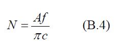
This means that as the beam diameter A [mm2] gets smaller, the length of the Near Field is smaller and similarly is with the frequency f [Hz]. Table B.1 demonstrates these dependencies.
According to the above numerical analysis, the depth of the NF decreases with frequency and also with the diameter of the beam. By applying a beam diameter of 1mm at a frequency of 20 MHz, the length of the NF is already at the value of ‘loosening decision’. Moreover, the application of a US transducer with a built-in beam diameter of 1mm will make the system simpler and without an intensity loss while narrowing the beam.
Acknowledgment: Our special thanks to Prof. Dan Adam from the Dept. of Biomedical Eng., The Technion I.I.T., for his encouragement and important remarks throughout discussions.
Table B1: Near field zone (N) as a function of frequency (f), The Tr/Rc aperture (D), and the Measured Resolution.
| Frequency | Wavelength | N|D=10‑2m | N|D=510-3m | N|10-3m | Measured Resolution |
|---|---|---|---|---|---|
| f | λ | λ/100 | |||
| Hz | mm | 10-3m | 10-3m | 10-3m | mm |
| 10MHz | 1.5 10-4 | 166 | 41.66 | 1.66 | 1.5* |
| 15MHz | 10-4 | 256 | 62.5 | 2.5 | 1* |
| 20MHz | 75 10-6 | 333 | 83 | 3.33 | 0.75* |
| 300KHz | 5 10-3 | 5 | 1.25 | 0.05 | 0.125** |
*Pulsed method.
** It is a Modulated US Continues Wave (MUSCW), with a modulation frequency
fmod. = 3 104 Hz, thus λ/400 = 0.125 mm.