
Journal of Clinical Images and Medical Case Reports
ISSN 2766-7820
Research Article - Open Access, Volume 4
Comparison of angular cephalometric measurements between CBCT mid-sagittal plane projections and conventional lateral cephalometric radiographs
Gan Lei1ⴕ; Chen Jieyu1,2ⴕ; Liu Chao1; Yu Rongcheng1; Li Chenghang3; She Yangyang2; Gao Feng3,4,5; Cao Yang1*
11Department of Orthodontics, Hospital of Stomatology, Sun Yat-sen University, Guangzhou, Guangdong Province, 510055, China.
22Department of Stomatology, the The Sixth Affiliated Hospital, Sun Yat-sen University, Guangzhou, Guangdong Province, 510655, China.
33Department of Colorectal Surgery, The Sixth Affiliated Hospital, Sun Yat-sen University, Guangzhou, Guangdong Province, 510655, China.
44Guangdong Institute of Gastroenterology, Guangzhou, Guangdong Province, 510655, China.
5Guangdong Provincial Key Laboratory of Colorectal and Pelvic Floor Diseases, The Sixth Affiliated Hospital, Sun Yat-sen University, Guangzhou, Guangdong Province, 510655, China.
ⴕThese authors contributed to the work equllly and should be regarded as co-first authors.
*Corresponding Author : Cao Yang
Doctor of Orthodontics, Professor, Department of Orthodontics, Hospital of Stomatology, Guanghua School of Stomatology, Sun Yat-Sen University, 56 Lingyuan Xi Rd. Guangzhou, Guangdong Province, 510055, China.
Email: caoyang@mail.sysu.edu.cn
Received : Dec 27, 2022
Accepted : Jan 19, 2023
Published : Jan 26, 2023
Archived : www.jcimcr.org
Copyright : © Yang C (2023).
Abstract
The purpose of this study was to verify the angular measurement values of conventional Lateral Cephalometric Radiographs (LCRs) and Cone-Beam Computed Tomography (CBCT) Mid- Sagittal Plane (MSP) projections when using the same cephalometric analysis method.
Methods: CBCT images and LCRs of 43 patients were randomly selected. Thirty-three landmarks were manually located on CBCT scans three times by two experienced operators. The landmarks were projected on to five Mid-Sagittal Planes (MSPs). Intraclass Correlation Coefficients (ICCs) were calculated to verify the reliability and reproducibility of landmark identification in CBCT images and angular measurements in LCRs. Paired t tests, correlation coefficients and Bland–Altman analyses were performed to compare thirteen angular measurement values between the LCR and CBCT MSP projections.
Results: Landmark identifications on CBCT images show excellent reliability, with intra and inter observer ICCs mostly larger than 0.9. For the comparison of angular measurements, there were no significant differences among the five MSP groups. LCR and CBCT MSP projections had a strong correlation, and although the mean of 11 measurements showed significant differences, the differences in the mean were trivial. The Bland-Altman analysis found a bias between the LCR and CBCT MSP projections.
Conclusions: CBCT analysis using midsagittal plane projections is a stable and useful method. This approach seems to allow the use of 2D LCR normative values in most angular measurements in CBCT MSP projections. The measurements where one or more landmarks lay far from the MSP showed distortions.
Keywords: Cephalometry; Mid-sagittal plane; CBCT; Orthodontics; Tomography; X-ray diagnosis.
Abbreviations: LCR: Lateral Cephalometric Radiograph; CBCT: Cone-Beam Computed Tomography; MSP: Mid-Sagittal Plane; ICC: Intraclass Correlation Coefficient; 2D: Two-Dimensional; 3D: Three-Dimensional; DICOM: Digital Imaging and Communication in Medicine; MPR: Multi-Planar Reconstruction; SEM: Standard Errors of Measurement; CI: Confidence Intervals.
Citation: Marinova L, Georgiev R, Evgeniev N. Clinical observations in three clinical cases with locally advanced chordomas. What is needed for early diagnosis with improved survival?. J Clin Images Med Case Rep. 2020; 1(1): 1005.
Introduction
Since the invention of the cephalometer by B. Holly Broadbent in 1930 [1], conventional lateral cephalometry has been the standard for the evaluation and orthodontic diagnosis of maxillofacial deformity [2]. Lateral Cephalometric Radiographs (LCR) depict a projection of the entire craniofacial structures onto a sagittal Two-Dimensional (2D) plane and provide a measurable assessment of themaxilla, mandible, and dentition and their spatial relationships in the anteroposterior and vertical dimensions [3]. The diagnostic information from these imaging modalities is considered valuable for treatment planning, prediction of growth and treatment results, and evaluation of orthodontic and surgical outcomes [4].
However, cephalometric measurements have intrinsic limitations. A Three-Dimensional (3D) anatomical structure flattened on a sagittal plane presents distortions and superimpositions of bony structures [5]. It is difficult to achieve accurate identification due to landmark overlap. Differential magnification of bilateral structures as result of a projective imaging geometry also leads to imperfect superimposition of landmarks [4]. Many studies have been published on errors associated with landmark identification, errors arising from the registration of landmarks, and errors due to measurement procedures [6-9]. Early cephalometers used separate X-ray heads to take the lateral and frontal views. Since both radiographs were taken without moving the subject’s head, mathematical methods could be used to derive the 3D measurements. However, market forces quickly eliminated the two X-ray head designs by using one source and moving the patient’s head 90 degrees to obtain either the posteroanterior or lateral view. Movement of the head between views was unavoidable, and the ability to create the third dimension mathematically was lost [10].
Cone-Beam Computed Tomography (CBCT) was introduced to the dental profession at the beginning of the 21st century [1]. The development of CBCT allowed precise 3D imaging to be obtained with consistently less radiation than conventional CT scans [5]. CBCT images can be assessed in all three planes of space, on images with life-size magnification, and without distortion or overlapping structures [11]. Furthermore, head position is not critical for 3D image capture and analysis; the spatial relationship among the various points is not changed in any way by variations in head orientation [12]. These features provide ease of landmark identification and precise superimposition of serial images [13]. Moreover, CBCT data sets can be imported as digital imaging and communication in medicine (DICOM) files into personal computer–based software to provide 3D reconstruction of the craniofacial skeleton [14].
When a CBCT scan is indicated for mixed reasons, cephalometric assessments can be performed directly on CBCT scans with a distortion-free procedure. If one projection provides the possibility of solving several diagnostic problems, it will replace registration from several projections in favor of one CBCT image [15]. However, CBCT-derived 3D cephalometry cannot yet replace the widely used LCR due to insufficient studies of normative value data [16]. It is highly unlikely that in the near future, 3D data from a large sample of untreated individuals with ideal occlusions that can be used to establish normative values for 3D assessments will become available due to examination costs and obvious ethical considerations [17]. Correspondence between CBCT and LCR needs to be determined during this transition period [4].
In some studies, LCR images extracted from 3D-CBCT data were compared with those obtained using conventional LCR [4,2,16]. A cephalometric similar to the traditional 2D cephalometric could be constructed with commercial software, but the problem of overlapping marker points remained. In other studies, landmarks were chosen directly from a CBCT image, without conversion to a 2Di mage, and these were then compared with those of conventional LCR [17-19]. It is recommended to identify landmarks in the MPR images. Landmarks could be identified without overlap. However, the landmarks on CBCT and LCR may be in consisten [20].
The aims of this study were to [1] examine the reliability and validity of landmark identification in CBCT; [2] validate the concordance of angular measurement values when the same cephalometric analysis method was used for conventional LCR and CBCT Mid-Sagittal Plane (MSP) projections; and [3] investigate the effect of different MSP projections on changes in angular measurements.
Materials and methods
Radiological image acquisition and processing
This retrospective study was approved by the Ethics Committee of Guanghua School of Stomatology, Hospital of Stomatology, Sun Yat-sen University (GHKQ-202205-L1). This study included [43] patients (21 male, 22 female, aged14-32 years). The CBCT scans and LCR swere retrospectively selected from the Department of Orthodontics between 2019 and 2022. All patients presented full permanent dentition apart from the third molar. Each patient had no dental treatment performed during interval between the CBCT and LCR, which was no more than a week.
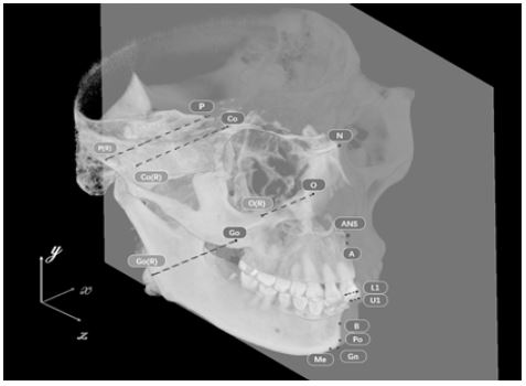
The CBCT scan images were saved as DICOM files. Mimics Research® software was used to reconstruct DICOM files into 3D images for landmark identification. The cephalometric landmarks used in the study are given in Table 1 and Figure 1.
Table 1: Definitions of cephalometric landmarks used used in two-dimensional (2D) and three-dimensional (3D) images.
| Landmark | Anatomical definition |
|---|---|
| Sella turcica (S) | Anterposterior midpoint of the pituitary fossa of the sphenoid bone |
| Nasion (Na) | Most anterior point of the frontonasal suture |
| Basion (Ba) | Most anterior point of the foramen magum |
| Porion (P) | Uppermost and midpoint of the external right roof of the auditory meatus |
| Pogonion (Po) | Most anterior point of the mandibular symphsis |
| Gnathion (Gn) | Most anteroinferior point of the mandibular symphysis |
| Me (Menton) | Lowest point of the mandibular symphsis |
| Anterior nasal spine (ANS) | Most anterior point of the maxillary process in the nasal floor region |
| Posterior nasal spine (PNS) | Most posterior and midpoint of the palatine bone contour |
| Gonion (Go) | Most poserior point of the posterior edge of the right branch. Bisection of the tangents of the poterior edge of the branch and the lower body |
| Orbital (O) | Most anterosuperior point of the infraorbital margin of the right orital |
| Incisal edge of central incisor (U1) | Lowest point of the incisal edge of the U1 |
| Apical root of upper central incisor (U1R) | Uppest point of the apical root of the U1 |
| Incisal edge of lower central incisor (L1) | Uppest point of the incisal edge of the L1 |
| Apical root of lower right central incisor (L1R) | Lowest point of the root of the L1 |
| Point A (A) | Most posterior point of the maxillarcurvtature, between the anterior nasal spine and the supradental point |
| Point B (B) | Most posterior point of the anterior surface of the mandibular symphysis |
| Crista galli (Cg)* | Middle point of crista galli |
| Incisive foramen (IF)* | The anteroposterior and mediolateral center of the incisive foramen |
| Condyle (Cd) | The most superior point of the condyle |
| Foramen spinosum (FS)* | the axial center of the area of the foramen spinosum at its most superior point as it joins the cranial fossa |
| Zygomaticofrontal suture (Z)* | medial point on the orbital rim of the zygomaticofrontal suture |
*These landmarks were used to reconstruct the MSP which were not identified in LCRs.
The patients’ identities were blinded during the export procedure. Two students (examiner a and examiner b) were trained by one experienced orthodontist on landmarks identification and marking. After that they performed landmark identification on both CBCT and conventional cephalogram separately. Each examiner went through these process three times, indicating landmarks in the Multi-Planar Reconstruction (MPR) views and then checking them on the 3D surface. The retest was performed at approximately the same time of the day on a subsequent day within a period of one week after the first session. For each session and each CT scan, the results were exported as an.xml file containing the x-, y-, z- coordinates of each landmark.
Ebraceph software (version 2.0, Riton Biomaterial Company, Guangzhou, China) was used for cephalometric tracings of the 2D images. LCR measurements were performed twice by the two examiner one week apart. When bilateral structures were not aligned or when the magnification difference between left and right structures was obvious, the operator chose the midpoint between the two structures.
On the CBCT, 32 3D cephalometric hard tissue landmarks were identified: 12 landmarks located in the median plane (unpaired landmarks) and 20 landmarks on either side of this plane (paired landmarks). 23 of the 32 landmarks had corresponding landmarks on conventional cephalograms. The other 9 landmarks (Z (left and right), IF, FS (left and right), Cg (left and right)) were used to reconstruct the MSP. 18 landmarks were identified on the conventional LCR and used to perform angular measurements.
The mid-sagittal planes were set using the following 5 methods (Figure 2).
Method 1: The midsagittal plane, including Ba, N and ANS, was set (Figure 2a).
Method 2: The midsagittal plane, including Ba, N and IF, was set (Figure 2b).
Method 3: The horizontal plane included the midpoint of each foramen spinosum (ELSA) and right/left bilateral porion, and the midsagittal plane was defined perpendicularly to the horizontal plane, passing through point Ba and ELSA (Figure 2c).
Method 4: The midsagittal plane crossed the N point (the midpoint of the nasofrontal suture) perpendicular to the FZ suture line. The FZ line was the line that connected the bilateral Z points (Figure 2d).
Method 5: The horizontal plane including right/left bilateral O and right Po, the MSP was defined perpendicularly to the horizontal plane, passing through Cg and Ba (Figure 2e).
The MSPs were set through the 5 methods described above. The measuring point was projected onto the MSP, and a parameter identical to that in the LCR was measured (Table 2). The bilateral measuring points were measured after designating the left and right measuring points using the midpoint between these 2 points. The coordinates of the projections and the angular measurements were both calculated by Python software (version 2.7.7; Python Software Foundation; Beaverton, Ore).
Statistical analysis
The Intra class Correlation Coefficient (ICC) obtained by comparing the values of x, y, and z, which indicate the exact location of each point on the axial, coronal and sagittal axes of the skull, was calculated to assess the reliability of the measurements. The values from conventional LCR analysis were used to calculate the intra examiner ICC, and the average value of two sets of cephalometric analysis from each examiner was used to calculate the inter examiner ICC. The values of intra- and inter examiner ICCs were interpreted according to Cicchetti and Sparrow [21] [0; 0.40] poor, [0.40; 0.60) fair, [0.60; 0.75) good, and [0.75; 1.0] excellent reliability.
The mean value and standard deviation of each measurement were computed separately for 3D and 2D values. Standard Errors Of Measurement (SEM) and 95% Confidence Intervals (CI) were calculated. The normality of the data was tested using the Shapiro‒Wilk test. The results of angular measurements on 5 MSP projections were evaluated statistically by Analysis Of Variance (ANOVA) and verified by post hoc analysis with Tukey’s multiple comparisons procedure. The angle between every two MSPs was calculated.
To compare the LCR and CBCT MSP projection measurements, paired t tests, correlation coefficients and Bland–Altman analysis were performed. All data were analyzed using the software R Studio (v. 4.1.3, R Studio PBC, Boston, MA, USA).
Results
Table 3 shows the intra examiner and inter examiner reliability test results for each CBCT landmark’s coordinate on the x, y, and z axes. Both examiners’ Intra examiner ICC values indicated excellent reliability for all landmarks of their marking (ICC ≥ 0.75). The values of Inter examiner ICC shown fairly good reliability in the x coordinates of points Co (L) and O (R) (0.60 ≥ ICC > 0.75) while other landmark coordinates had excellent reliability (ICC ≥ 0.75).
For all LCR measurements, intra examiner and inter examiner reliability were excellent. Table 4 shows that the intra examiner ICC ranged from 0.92 to 0.99 for all angular measurements, and the inter examiner ICC ranged from 0.91 to 0.99 for all angular measurements.
The Shapiro-Wilk test (p > 0.05) was used to confirm that the angular measurement data had a normal distribution. For each group, the means, standard deviations, standard errors, and 95% confidence intervals were calculated (Table 5). The results of 5 CBCT MSP projections were statistically evaluated using Analysis Of Variance (ANOVA) and confirmed using post hoc analysis with Tukey’s multiple comparisons procedure. There were no statistically significant differences between the 5 MSP groups.
The angles between every two MSPs ranged from 0.63±0.58 degrees to 4.15 ± 2.67 degrees (Table 6).
Table 2: Description of angular measurements used in this study.
| Angular measurements | Definition |
|---|---|
| SNA | Angle between point S, point Na, and point A |
| SNB | Angle between point S, point Na, and point B |
| ANB | Angle between point A, point Na, and point B |
| AB-NPo | A-B plane to facial plane angle |
| FH-NPo | Facial angle |
| SGn-FH | Y-axis, FH plane-SGn angle |
| NA-APo | Angle of convexity |
| FMA (MP-FH) | Angle between mandibular plane to Frankfurt horizontal line (Porion to Orbitale) |
| U1-SN | Angle between most proclined upper central incisor long axis to Sella-Nasion line |
| U1-NA | Angle between most proclined upper central incisor long axis to Nasion-A point line |
| L1-NB | Angle between most proclined lower central incisor long axis to Nasion-B point line |
| U1-L1 | Angle between U1-U1r line and L1-L1rroot line |
| IMPA (L1-MP) | Angle between most proclined lower central incisor long axis to Mandibular plane |
There was a statistically significant difference between LCR and CBCT MSP projections for most of the measurements (Table 7). Although the average difference for these measurements between the 2 methods was statistically significant (P < 0.05), for most of them (SNA, SNB, ANB, FH-NPo, SGn-FH, NA-APo, AB-NPo, U1-SN, IMPA-L1, U1-NA), The actual mean average difference ranged from 0.24° to 1.56°, which is comparable to or less than the measurement standard error. The disparity between CBCT MSP projections and LCR for the angular measurements (FMA, L1-NB, U1-L1) was greater than their standard error.

On analyzing the correlations of each of the variables for the LCR and CBCT MSP projections, no angular measurement was found to show a statistically difference, and the correlations between the LCR and CBCT MSP projections are high range between 0.74 to 0.95 (Table 8).
Bland‒Altman analysis evaluates the agreement between two sets of measurements, and it is usually applied in a clinical context to compare a new measurement method to a gold standard.
The Shapiro Wilk test was used to analyse the normality of differences, and the differences between LCR and CBCT MSP projections were normally distributed in FH-Npo, SGn - FH, FMA, AB - NPo, L1-MP, L1-NB and U1-L1. Figure 3 depicts exemplary Bland-Altman plots of FH-Npo, SGn-FH, FMA, AB - NPo, L1-MP, L1-NB and U1-L1. Only the Bland-Altman mean difference demonstrated a minimal and clinically acceptable bias for SGn-FH. Even though the correlation between the angular measurements of LCR and CBCT MSP projections was good, the Bland Altman analysis revealed a bias between the two sets.
Table 3: Reliability testing of CBCT landmarks marking on each coordinate axis through inter examiner and intra examiner ICC.
| landmark | Intra examiner reliability | Intra examiner reliability | Intra examiner reliability | ||||||
|---|---|---|---|---|---|---|---|---|---|
| Examiner a | Examiner b | ||||||||
| X | Y | Z | X | Y | Z | X | Y | Z | |
| A | >0.99 | >0.99 | >0.99 | >0.99 | >0.99 | >0.99 | >0.98 | >0.99 | >0.99 |
| ANS | >0.99 | >0.99 | >0.99 | >0.99 | >0.99 | >0.99 | 0.97 | 0.99 | >0.99 |
| B | >0.99 | >0.99 | >0.99 | >0.99 | >0.99 | >0.99 | 0.99 | >0.99 | 0.98 |
| Ba | >0.99 | >0.99 | >0.99 | 0.94 | >0.99 | >0.99 | 0.96 | >0.99 | >0.99 |
| Co (L) | >0.99 | >0.99 | >0.99 | >0.99 | >0.99 | >0.99 | 0.75 | 0.96 | >0.99 |
| Co (R) | >0.99 | >0.99 | >0.99 | >0.99 | >0.99 | >0.99 | 0.77 | 0.95 | >0.99 |
| Gn | >0.99 | >0.99 | >0.99 | >0.99 | >0.99 | 0.91 | 0.97 | >0.99 | 0.98 |
| Go (L) | >0.99 | >0.99 | >0.99 | >0.99 | >0.99 | >0.99 | 0.99 | 0.98 | 0.99 |
| Go (R) | >0.99 | >0.99 | >0.99 | >0.99 | >0.99 | >0.99 | 0.99 | 0.98 | 0.99 |
| IF | >0.99 | >0.99 | >0.99 | >0.99 | >0.99 | >0.99 | 0.99 | >0.99 | >0.99 |
| L1 (L) | >0.99 | >0.99 | >0.99 | >0.99 | >0.99 | >0.99 | 0.99 | >0.99 | >0.99 |
| L1 (R) | >0.99 | >0.99 | >0.99 | >0.99 | >0.99 | >0.99 | 0.99 | >0.99 | >0.99 |
| L1R (L) | >0.99 | >0.99 | >0.99 | >0.99 | >0.99 | >0.99 | 0.97 | >0.99 | >0.99 |
| L1R (R) | >0.99 | >0.99 | >0.99 | >0.99 | >0.99 | >0.99 | 0.97 | >0.99 | >0.99 |
| Me | >0.99 | >0.99 | >0.99 | >0.99 | >0.99 | >0.99 | 0.96 | >0.99 | >0.99 |
| N | >0.99 | >0.99 | >0.99 | >0.99 | >0.99 | >0.99 | 0.94 | >0.99 | 0.99 |
| O (L) | >0.99 | >0.99 | >0.99 | 0.99 | >0.99 | >0.99 | 0.79 | 0.99 | >0.99 |
| O (R) | >0.99 | >0.99 | >0.99 | 0.97 | >0.99 | >0.99 | 0.64 | 0.97 | >0.99 |
| P (L) | >0.99 | >0.99 | >0.99 | 0.99 | >0.99 | >0.99 | 0.87 | 0.99 | >0.99 |
| P (R) | >0.99 | >0.99 | >0.99 | 0.99 | >0.99 | >0.99 | 0.93 | 0.99 | >0.99 |
| PNS | >0.99 | >0.99 | >0.99 | >0.99 | >0.99 | >0.99 | 0.99 | 0.99 | >0.99 |
| Po | >0.99 | >0.99 | >0.99 | 0.99 | >0.99 | >0.99 | 0.97 | >0.99 | >0.99 |
| S | >0.99 | >0.99 | >0.99 | >0.99 | >0.99 | >0.99 | 0.94 | >0.99 | >0.99 |
| U1 (L) | >0.99 | >0.99 | >0.99 | >0.99 | >0.99 | >0.99 | 0.96 | >0.99 | >0.99 |
| U1 (R) | >0.99 | >0.99 | >0.99 | 0.99 | >0.99 | >0.99 | 0.93 | >0.99 | >0.99 |
| U1R (L) | >0.99 | >0.99 | >0.99 | >0.99 | >0.99 | >0.99 | 0.88 | >0.99 | >0.99 |
| U1R (R) | >0.99 | >0.99 | >0.99 | >0.99 | >0.99 | >0.99 | 0.89 | >0.99 | >0.99 |
Table 4: Reliability testing of tracing measurement on LCR through inter examiner and intra examiner ICC.
| Angular measurements | Intra examiner reliability | Intra examiner reliability | Inter examiner reliability |
|---|---|---|---|
| Examiner a | Examiner b | ||
| SNA | 0.99 | 0.99 | 0.91 |
| SNB | >0.99 | >0.99 | 0.99 |
| ANB | 0.99 | 0.92 | 0.89 |
| AB-NPo | 0.99 | 0.94 | 0.90 |
| FH-NPo | 0.98 | 0.99 | 0.92 |
| SGn-FH | 0.98 | 0.99 | 0.92 |
| NA-APo | 0.99 | 0.94 | 0.92 |
| FMA (MP-FH) | 0.99 | >0.99 | 0.96 |
| U1-SN | 0.98 | >0.99 | 0.99 |
| U1-NA | 0.97 | 0.97 | 0.98 |
| L1-NB | 0.99 | >0.99 | 0.99 |
| U1-L1 | 0.92 | 0.95 | 0.96 |
| L1-MP | 0.99 | >0.99 | 0.99 |
Table 5: The course of endoscopic treatments.
| Measurement | 2D LCR | MSP1 | MSP2 | MSP3 | MSP4 | MSP4 | ||||||||||||||||||
|---|---|---|---|---|---|---|---|---|---|---|---|---|---|---|---|---|---|---|---|---|---|---|---|---|
| mean | SD | SE | 95% CI | mean | SD | SE | 95% CI | mean | SD | SE | 95% CI | mean | SD | SE | 95% CI | mean | SD | SE | 95% CI | mean | SD | SE | 95% CI | |
| SNA | 81.71 | 3.48 | 0.53 | (80.64, 82.78) | 82.85 | 3.51 | 0.54 | (81.77, 83.93) | 82.85 | 3.52 | 0.54 | (81.77 , 83.94 ) | 82.75 | 3.56 | 0.54 | (81.66 , 83.85 ) | 82.86 | 3.52 | 0.54 | (81.78 , 83.94 ) | 82.84 | 3.52 | 0.54 | (81.76 ,83.92 ) |
| SNB | 78.87 | 4.96 | 0.76 | (77.35 , 80.40) | 79.12 | 4.88 | 0.74 | (77.62, 80.62) | 79.12 | 0.74 | 0.74 | (77.62 , 80.62 ) | 79.03 | 4.86 | 0.74 | (77.53 , 80.52 ) | 79.13 | 4.87 | 0.74 | (77.63 ,80.63 ) | 79.11 | 4.88 | 0.74 | (77.61 ,80.62 ) |
| ANB | 2.83 | 3.21 | 0.49 | (1.84 , 3.82) | 3.73 | 3.84 | 0.59 | (2.55, 4.91) | 3.73 | 0.59 | 0.59 | (2.55 , 4.91 ) | 3.72 | 3.84 | 0.59 | (2.54 , 4.91 ) | 3.73 | 3.83 | 0.58 | (2.55 ,4.91 ) | 3.72 | 3.84 | 0.59 | (2.54 ,4.91 ) |
| FH-NPo | 87.51 | 3.90 | 0.59 | (86.31 , 88.71) | 87.95 | 3.55 | 0.54 | (86.31 ,88.71) | 87.95 | 0.54 | 0.54 | (86.85 , 89.04 ) | 87.87 | 3.51 | 0.54 | (86.78 ,88.95 ) | 87.95 | 3.55 | 0.54 | (86.86 ,89.04 ) | 87.94 | 3.55 | 0.54 | (86.85 ,89.03 ) |
| SGn-FH | 62.57 | 3.71 | 0.57 | (61.42 , 63.71) | 61.47 | 3.52 | 0.54 | (60.38,62.55) | 61.47 | 0.54 | 0.54 | (60.39 ,62.55 ) | 61.60 | 3.47 | 0.53 | (60.53 ,62.67 ) | 61.46 | 3.52 | 0.54 | (60.38 ,62.55 ) | 61.48 | 3.52 | 0.54 | (60.40 ,62.56 ) |
| NA-APo | 5.89 | 7.51 | 1.15 | (3.58, 8.20) | 7.17 | 8.33 | 1.27 | (4.60,9.73) | 7.16 | 1.27 | 1.27 | (4.59 ,9.73 ) | 7.17 | 8.34 | 1.27 | (4.60 ,9.74 ) | 7.17 | 8.32 | 1.27 | (4.61 ,9.73 ) | 7.15 | 8.34 | 1.27 | (4.58 ,9.71 ) |
| FMA(MP-FH) | 28.28 | 5.51 | 0.84 | (26.59 , 29.98) | 24.78 | 4.96 | 0.76 | (23.25,26.3) | 24.78 | 0.76 | 0.76 | (23.25 ,26.30 ) | 24.84 | 4.97 | 0.76 | (23.31 ,26.37 ) | 24.78 | 4.96 | 0.76 | (23.25 ,26.30 ) | 24.79 | 4.96 | 0.76 | (23.26 ,26.31 ) |
| AB-NPo | -4.33 | 5.14 | 0.78 | (-5.91 , -2.74) | -5.24 | 5.25 | 0.80 | (-6.86,-3.63) | -5.24 | 0.80 | 0.80 | (-6.86 ,-3.63 ) | -5.25 | 5.23 | 0.80 | (-6.85 ,-3.64 ) | -5.24 | 5.24 | 0.80 | (-6.85 ,-3.63 ) | -5.23 | 5.26 | 0.80 | (-6.85 ,-3.61 ) |
| U1-SN | 104.64 | 10.41 | 1.59 | (101.43 , 107.84) | 104.10 | 10.64 | 1.62 | (100.83,107.37) | 104.10 | 1.62 | 1.62 | (100.83 ,107.38 ) | 103.94 | 10.55 | 1.61 | (100.69 ,107.18 ) | 104.12 | 10.65 | 1.62 | (100.84 ,107.40 ) | 104.09 | 10.63 | 1.62 | (100.82 ,107.37 ) |
| IMPA-L1-MP- | 94.31 | 8.18 | 1.25 | (91.79 , 96.83) | 93.70 | 8.72 | 1.33 | (91.01,96.38) | 93.70 | 1.33 | 1.33 | (91.01 ,96.38 ) | 93.67 | 8.78 | 1.34 | (90.97 ,96.38 ) | 93.68 | 8.75 | 1.33 | (90.99 ,96.38 ) | 93.68 | 8.76 | 1.34 | (90.98 ,96.37 ) |
| U1-NA | 22.87 | 9.31 | 1.42 | (20.01 , 25.74) | 21.31 | 9.59 | 1.46 | (18.36,24.26) | 21.31 | 1.46 | 1.46 | (18.36 ,24.27 ) | 21.25 | 9.54 | 1.45 | (18.31 ,24.18 ) | 21.31 | 9.60 | 1.46 | (18.36 ,24.27 ) | 21.31 | 9.59 | 1.46 | (18.36 ,24.26 ) |
| L1-NB | 30.01 | 8.03 | 1.22 | (27.53 , 32.48) | 26.34 | 7.04 | 1.07 | (24.18,28.51) | 26.35 | 1.07 | 1.07 | (24.19 ,28.51 ) | 26.35 | 6.97 | 1.06 | (24.21 ,28.50 ) | 26.35 | 7.01 | 1.07 | (24.19 ,28.51 ) | 26.34 | 7.02 | 1.07 | (24.18 ,28.50 ) |
| U1-L1 | 124.20 | 11.90 | 1.81 | (120.53, 127.86) | 129.00 | 12.34 | 1.88 | (125.21,132.8) | 129.00 | 1.88 | 1.88 | (125.20 ,132.80) | 129.10 | 12.36 | 1.88 | (125.30 ,132.90 ) | 129.00 | 12.35 | 1.88 | (125.20,132.80 ) | 129.02 | 12.35 | 1.88 | (125.22,132.83) |
SD: Standard Deviations; SE: Standard Error; CI: Confidence Interval; 2D: Two-Dimensional; MSP CBCT: MSP Projections.
Table 6: The angles between two MSP planes (°).
| MSP | mean | SD |
|---|---|---|
| MSP1 VS MSP2 | 0.63 | 0.58 |
| MSP1 VS MSP3 | 3.82 | 2.39 |
| MSP1 VS MSP4 | 2.02 | 1.00 |
| MSP1 VS MSP5 | 1.77 | 0.93 |
| MSP2 VS MSP3 | 3.61 | 2.36 |
| MSP2 VS MSP4 | 1.73 | 0.96 |
| MSP2 VS MSP5 | 1.5 | 0.81 |
| MSP3 VS MSP4 | 4.15 | 2.67 |
| MSP3 VS MSP5 | 3.35 | 2.19 |
| MSP4 VS MSP5 | 2.07 | 1.22 |
MSP: Mid-Sagittal Plane; SD: Standard Deviation.
Table 7: The course of endoscopic treatments.
| Measurements | 2D vs MSP1 | 2D vs MSP2 | 2D vs MSP3 | 2D vs MSP4 | 2D vs MSP5 | |||||
|---|---|---|---|---|---|---|---|---|---|---|
| p value a | Rb | p value | R | p value | R | p value | R | p value | R | |
| ANB | < 0.01 | 0.74 | < 0.01 | 0.74 | < 0.01 | 0.74 | < 0.01 | 0.74 | < 0.01 | 0.74 |
| SNA | 0.01 | 0.91 | 0.01 | 0.91 | 0.01 | 0.91 | < 0.01 | 0.91 | 0.01 | 0.91 |
| SNB | 0.44a | 0.88 | 0.44a | 0.88 | 0.63a | 0.88 | 0.42a | 0.88 | 0.45a | 0.88 |
| AB-NPo | 0.01 | 0.93 | 0.01 | 0.93 | 0.01 | 0.93 | 0.01 | 0.94 | 0.01 | 0.93 |
| FH-Npo | < 0.01 | 0.93 | < 0.01 | 0.93 | < 0.01 | 0.93 | < 0.01 | 0.93 | < 0.01 | 0.93 |
| SGn-FH | < 0.01 | 0.91 | < 0.01 | 0.91 | < 0.01 | 0.90 | < 0.01 | 0.91 | < 0.01 | 0.90 |
| NA-APo | 0.02 | 0.95 | 0.02 | 0.95 | 0.02 | 0.95 | 0.02 | 0.95 | 0.03 | 0.95 |
| FMA | < 0.01 | 0.90 | < 0.01 | 0.90 | < 0.01 | 0.90 | < 0.01 | 0.90 | < 0.01 | 0.90 |
| U1-SN | 0.09 | 0.93 | 0.09 | 0.93 | 0.03 | 0.93 | 0.10 | 0.93 | 0.09 | 0.93 |
| U1-NA | 0.01 | 0.86 | 0.01 | 0.86 | 0.01 | 0.86 | 0.01 | 0.86 | 0.01 | 0.86 |
| L1-NB | < 0.01 | 0.92 | < 0.01 | 0.92 | < 0.01 | 0.92 | < 0.01 | 0.92 | < 0.01 | 0.92 |
| U1-L1 | < 0.01 | 0.81 | < 0.01 | 0.81 | < 0.01 | 0.80 | < 0.01 | 0.80 | < 0.01 | 0.80 |
| L1-MP | 0.38a | 0.92 | 0.38a | 0.92 | 0.37a | 0.92 | 0.37a | 0.92 | 0.37a | 0.92 |
aStatistical significance (P>0.05).
bStrength of correlation coefficient (R) is estimated as follows: 0.8–1 (very strong), 0.6–0.79 (strong), 0.4–0.59 (moderate), 0.2–0.39 (weak), and 0–0.19 (very weak
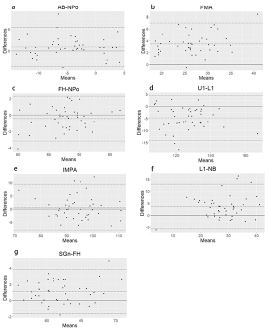
Table 8: Bland–Altman analysis performed on LCR and CBCT MSP projections.
| Measurements | 2D VS MSP1 | 2D VS MSP2 | 2D VS MSP3 | 2D VS MSP4 | 2D VS MSP5 | ||||||||||
|---|---|---|---|---|---|---|---|---|---|---|---|---|---|---|---|
| bias | SD of bias | LoA | bias | SD of bi | LoA | bias | SD of bias | LoA | bias | SD of bias | LoA | bias | SD of bias | LoA | |
| AB-NPo | 0.90 | 2.29 | (-3.59, 5.39) | 0.91 | 2.28 | (-3.56,5.38) | 0.92 | 2.31 | (-3.61,5.45) | 0.92 | 2.28 | (-3.56,5.39) | 0.92 | 2.28 | (-3.56,5.40) |
| ANB | -0.90 | 1.84 | (-4.5, 2.70) | -0.90 | 1.84 | (-4.50,2.70) | -0.89 | 1.85 | (-4.51,2.72) | -0.90 | 1.83 | (-4.49,2.69) | -0.89 | 1.84 | (-4.50,2.71) |
| FH-Npo | -0.43 | 1.39 | (-3.16, 2.30) | -0.44 | 1.38 | (-3.15,2.27) | -0.35 | 1.39 | (-3.09,2.38) | -0.43 | 1.39 | (-3.17,2.30) | -0.44 | 1.40 | (-3.18,2.30) |
| FMA | 3.49 | 1.79 | (-0.02,7.01) | 3.50 | 1.79 | (0.00,7.01) | 3.44 | 1.77 | (-0.04,6.91) | 3.50 | 1.78 | (0.01,6.99) | 3.51 | 1.78 | (0.01,7.00) |
| SGn-FH | 1.09 | 1.39 | (-1.64,3.81) | 1.10 | 1.38 | (-1.61,3.81) | 0.97 | 1.38 | (-1.74,3.68) | 1.10 | 1.39 | (-1.62,3.82) | 1.10 | 1.39 | (-1.63,3.83) |
| IMPA | 0.63 | 4.53 | (-8.25,9.51) | 0.62 | 4.53 | (-8.26,9.51) | 0.63 | 4.56 | (-8.31,9.57) | 0.61 | 4.53 | (-8.26,9.48) | 0.61 | 4.52 | (-8.24,9.47) |
| L1-NB | 3.67 | 4.80 | (-5.74,13.08) | 3.65 | 4.80 | (-5.75,13.06) | 3.65 | 4.82 | (-5.80,13.11) | 3.66 | 4.79 | (-5.73,13.04) | 3.66 | 4.78 | (-5.71,13.04) |
| NA-Apo | -1.26 | 3.56 | (-8.24,5.72) | -1.28 | 3.52 | (-8.17,5.61) | -1.28 | 3.60 | (-8.34,5.77) | -1.27 | 3.54 | (-8.21,5.67) | -1.28 | 3.54 | (-8.21,5.66) |
| SNA | -1.13 | 2.53 | (-6.08,3.82) | -1.15 | 2.52 | (-6.08,3.79) | -1.04 | 2.54 | (-6.03,3.95) | -1.14 | 2.52 | (-6.08,3.81) | -1.14 | 2.52 | (-6.08,3.81) |
| SNB | -0.24 | 2.06 | (-4.27,3.79) | -0.25 | 2.05 | (-4.27,3.77) | -0.15 | 2.08 | (-4.24,3.93) | -0.25 | 2.05 | (-4.26,3.77) | -0.24 | 2.05 | (-4.26,3.77) |
| U1-L1 | -4.83 | 4.78 | (-14.2,4.54) | -4.81 | 4.78 | (-14.18,4.57) | -4.91 | 4.79 | (-14.29,4.48) | -4.81 | 4.78 | (-14.17,4.56) | -4.81 | 4.77 | (-14.16,4.55) |
| U1-NA | 1.56 | 3.84 | (-5.96,9.08) | 1.56 | 3.86 | (-6.01,9.12) | 1.63 | 3.83 | (-5.88,9.13) | 1.56 | 3.84 | (-5.97,9.09) | 1.56 | 3.84 | (-5.97,9.10) |
| U1-SN | 0.54 | 3.82 | (-6.95,8.03) | 0.52 | 3.84 | (-7.01,8.05) | 0.70 | 3.80 | (-6.76,8.15) | 0.53 | 3.82 | (-6.96,8.02) | 0.54 | 3.82 | (-6.96,8.03) |
LoA: Limits of Agreement.
Discussion
Although 2D cephalometric analysis has been utilized in orthodontics for over a century, its inaccuracies have never ceased to be discussed. Conventional LCR analysis has problems with projective distortions and rotational errors, which may compromise the accuracy and reusability of recorded data [6,22]. Cephalometric measurements based on CBCT images have been developed and found to perform similarly to 2D cephalometric tracings. CBCT images reduce the problems of distortion and rotation, and globally efforts have been made to compare 2D and 3D cephalometric analysis [2,23,17]. There are multiple methods to synthesize 2D views from a CBCT image volume, and both orthogonal and perspective projections can be used with similar precision and accuracy as conventional cephalograms [4]. However, these methods did not consider the reference used by the reconstruction algorithm to define the mid sagittal plane. Due to the landmark overlap, accurate identification may still be challenging. In some studies, the landmarks were identified directly from a 3D-CBCT image without conversion to a 2D image and afterwards compared to those of conventional LCR. These methods still do not consider head orientation-induced changes in CBCT-generated images [17-19]. In this study, landmarks were identified in CBCT images and then projected onto the mid sagittal plane. The bilateral measuring points were measured after designating the left and right measuring points, using the midpoint between these 2 points. Angular measurements were performed by the projected points on the MSP. Therefore, landmark identification was performed directly in CBCT images without conversion. Head orientation was considered, and the head position was reproducible in future comparisons if needed.
To determine and compare the intra examiner and inter examiner reliabilities of commonly used cephalometric landmarks identified on CBCT images, this study performed landmark identification using MPR views and found that intra examiner and inter examiner reliabilities for all coordinates for the most of landmarks on CBCT images were greater than 0.90 (ICC value).Consistent with previous studies [24,25], The intra- and inter examiner reliability were both excellent, even though the ICC values of three x-coordinates (points O, Co, and P) were less than 0.90. Intraexaminer differences could be due to the nature of the cephalometric landmark, image quality, and blurring of anatomic structures, whereas inter examiner differences might be caused by variations in the examiner’s training and experience [7,9]. In this study, the examiners were orthodontic students who were trained and calibrated before the research to ensure that they were proficient with the software and identifying the landmarks. The landmarks O, Co, and P were not located on sharp edges, foramina, or sutures in the 3D images; instead, they were on surfaces and curves in the 3D depiction, making precise identification more difficult compared to other landmarks [26].
We evaluated the intra- and inter examiner reliabilities of angular parameters for traditional 2D cephalograms, and the ICC value suggested that the reliability was good, suggesting that two examiners are proficient in the procedure of LCR landmarks identification.
In recent years, the Mid-Sagittal Plane (MSP) has mostly been used in the diagnosis of facial asymmetry and computer-based preoperative planning [27,28]. In the ideal condition of 2D cephalographic projection, the sagittal plane of the patient should be perpendicular to the central ray of the beam and parallel to the film plane [22]. In practice, however, the alignment of the cephalographic system may differ from the theoretical ideal. In the CBCT synthesized cephalogram, the angular deviations foreshorten and skew the proportions of the resulting image [29,30]. Aside from being used for skull orientation, the MSP serves as a reference plane for both 3D cephalometric analysis and the superimposition of radiographs from different time points [29]. Therefore, the definition of the MSP was very important in the study of parametrics in both 2D and 3D. Some studies in the past have not clearly articulated the mid sagittal plane used in the measurement [2,26,19]. On the other hand, there is no gold standard for the precise MSP because the ideal MSP divides the skull into two mirror halves, while a real skull is never symmetrical [31]. Several techniques have been proposed to improve the accuracy and reliability of MSP localization, moving away from the traditional cephalometric approach and toward more complex methodologies such as morphometric methods and mirroring-and-registration methods [32]. Even though it is referred to as time computing, traditional cephalometry is the most common method used in practice.
We performed five MSPs, which were mentioned in a previous study [27-29,33,34] in this study. No clinically significant difference in angular measurements was observed among CBCT projections using these midsagittal planes. The results were consistent with the study of Jung et al [16] in which three MSPs were used to obtain the projections. In this study, the symmetry of patients’ skulls was not considered because our pilot study showed that different MSPs may lead to different diagnoses in borderline cases but also that asymmetric patterns vary among patients. Moreover, in the clinic, asymmetric patients are more inclined to undergo CBCT. It is more favorable for patients if cephalometric assessments can be performed directly on CBCT scans. We calculated the angles between MSPs for the patients, and the mean angles ranged from 0.63 ± 0.58 degrees to 4.15 ± 2.67 degrees. The difference between the mind sagittal planes was too small to cause a significant difference in angle measurements.
Previous studies compared the measurement values of the 3D cephalometric analysis of CBCT and 2D cephalometric analysis. Kumar et al. [4], Nalçaci et al [19], Natalia et al. [35], and Oliver et al [2] reported that there was no statistically significant difference in most of the linear and angular measurements between 2D and 3D methods. Li et al [36]. Analyzed the differences between CBCT and RLC cephalometric methods in 40 patients by means of a paired t test. The results indicated that the two methods showed significant differences in all measurements. In the present study, although the correlations between the 2D and MSPs are high, 11 of 13 angular measurements were significantly different between 2D and 3D projections by paired t test. In 8 of 11 angular measurements (SNA, ANB, FH- Npo, SGn-FH, NA-Apo, AB- Npo, U1-SN, IMPA-L1, U1-NA), the actual mean average difference ranged from 0.24 degrees-1.56 degrees, similar to or smaller than the standard error for the measurements. A paired t test detects systematic differences even if they are of low or no clinical significance. The correlation coefficient does not indicate the actual agreement between 2 measurements but only the strength of the relationship between 2 variables. For example, 2 measurements can have perfect correlation but never agree [37]. When we compared the methods of 2D and 3D, the most concern was whether the existing valves of two-dimensional measurements could be applied in 3D. Assuming 2 degrees as a potential threshold for clinically meaningful differences [26,16], the augmented measurements SNA,SNB, ANB, FH-Npo, SGn-FH, NA-Apo, AB-Npo, U1-SN, IMPA, and U1-NA were all within the clinically acceptable range of measurement error. The Bland‒Altman plot was intended to compare methods of clinical measurement. Baldiniet al. [5] demonstrated that between 2 and 3D measurements, further information could be obtained by Bland‒Altman analysis, providing useful information to assess the bias of the measurements to formulate educated guesses about their correction using specific algorithms to be investigated in future studies. In the present study, we performed Bland‒Altman analysis for 2D and 3D projections. To create what is thought of as a standard Bland‒Altman plot, the differences need to be normally distributed. Only the differences in FH-Npo, SGn-FH, AB-Npo, FMA, IMPA, L1-NB and U1-L1 were normally distributed. Bland–Altman analysis evidenced a bias between the two sets in these angular measurements (FMA, L1-NB, U1-L1). The biases were narrow in FH-Npo, SGn-FH, AB-Npo, and IMPA, but the Lo As were quite wide (-3.16° to 2.30°,-1.6° to 3.81°, -3.59° to 5.39°, and -8.25° to 9.51°). Lo Asseem un acceptable in AB-Npo and IMPA in the clinic.
The actual mean average difference or bias were smaller in angular measurements made by single landmarks on or near the MSPs than for those formed by paired landmarks. U1-L1 had the greatest bias, which may be because the landmark overlap in the 2D tracings generates huge measurement errors. The landmarks Go, Co, and P were located on flat or curved surfaces, making them difficult to precisely reference or define on CBCT images. There could be inconsistencies with the identification in 2D and 3D, which contributed to the bias of the measurement.
Conclusion
The landmark identification in 3D technology is equally reliable of clinical reliability. The angular measurements taken on CBCT projections using MSPs valid and reproducible. Utilizing the mid sagittal plane for CBCT analysis is a reliable and efficient method. It appears to permit the use of 2D LCR normative values for the most of angular measurements in CBCT projections. However, the measurements in which one or more landmarks lie far from the MSP bear distortions.
Author contributions
Gan Lei: First writer, Original Draft, Conducting the research and investigation process.
Chen Jieyu: Co-first writer, Development or design of methodology, application of statistical Review & Editing.
Liu Chao: Conducting the research and investigation process.
Yu Rongcheng: Conducting the research and investigation process.
Li Chenghang: Implementation of the computer code and supporting algorithms.
SheYang Yang: Data Curation.
Gao Feng: Co-Corresponding writer Ideas; formulation or evolution of overarching research goals and aims.
Cao Yang: Corresponding writer Ideas; formulation or evolution of overarching research goals and aims.
References
- Hans MG, Martin Palomo J, Valiathan M. History of imaging in orthodontics from Broadbent to cone-beam computed tomography. Am J Orthod Dentofacial Orthop. 2015; 148: 914-921.
- Van Vlijmen OJC, Bergé SJ, Swennen GRJ, Bronkhorst EM, Katsaros C, et al. Comparison of Cephalometric Radiographs Obtained From Cone-Beam Computed Tomography Scans and Conventional Radiographs. J Oral Maxillofac Surg. 2009; 67: 92-97.
- Scheide man GB, Bell WH, Legan HL, Finn RA, Reisch JS. Cephalometric analysis of dentofacial normals. Am J Orthod. 1980; 78: 404-420.
- Kumar V, Ludlow JB, Mol A, Cevidanes L. Comparison of conventional and cone beam CT synthesized cephalograms. Dentomaxillofacial Radiol. 2007; 36: 263-269.
- Baldini B, Cavagnetto D, Baselli G, Sforza C, Tartaglia GM. Cephalometric measurements performed on CBCT and reconstructed lateral cephalograms: A cross-sectional study providing a quantitative approach of differences and bias. BMC Oral Health. 2022; 22.
- Gravely JF, Benzies PM. The clinical significance of tracing error in cephalometry. Brit JOrthod. 1974; 1: 95-101.
- Baumrind S, Frantz RC. The reliability of head film measurements. Am J Orthod. 1971; 60: 505-517.
- MIDTGÅRD J, BJÖRK G, LINDER-ARONSON S. Reproducibility of Cephalometric Landmarks and Errors of Measurements of Cephalometric Cranial Distances. Angle Orthod. 1974; 44: 56-61.
- Savage AW, Showfety KJ, Yancey J. Repeated measures analysis of geometrically constructed and directly determined cephalometric points. Am J Orthod Dentofacial Orthop. 1987; 91: 295-299.
- Hans MG, Broadbent BH, Nelson SS. The Broadbent-Bolton Growth Study-past, present, and future. 1994; 1095: 598-603.
- van Bunningen RH, Dijkstra PU, Dieters A, van der Meer WJ, Kuijpers-Jagtman AM, et al. Precision of orthodontic cephalometric measurements on ultra low dose-low dose CBCT reconstructed cephalograms. Clin Oral Investig. 2022; 26: 1543-1550.
- Cevidanes L, Oliveira AEF, Motta A, Phillips C, Burke B, et al. Head orientation in CBCT-generated cephalograms. Angle Orthod. 2009; 79: 971-977.
- Chien PC, Parks ET, Eraso F, Hartsfield JK, et al. Comparison of reliability in anatomical landmark identification using two-dimensional digital cephalometrics and three-dimensional cone beam computed tomography in vivo. Dentomaxillofacial Radiol. 2009; 38: 262-273.
- Mozzo P, Procacci C, Tacconi A, Tinazzi Martini P, Bergamo Andreis IA, et al. A new volumetric CT machine for dental imaging based on the cone-beam technique: Preliminary results. Eur Radiol. 1998; 8: 1558-1564.
- Review AS. New Sagittal and Vertical Cephalometric Analysis Methods: A Systematic Review. Published online. 2022.
- Jung PK, Lee GC, Moon CH. Comparison of cone-beam computed tomography cephalometric measurements using a midsagit tal projection and conventional two-dimensional cephalometric measurements. Korean J Orthod. 2015; 45: 282-288.
- Gribel BF, Gribel MN, Manzi FR, Brooks SL, McNamara JA. From 2D to 3D: An algorithm to derive normal values for 3-dimensional computerized assessment. Angle Orthod. 2011; 81: 5-12.
- Zamora N, Llamas JM, Cibrián R, Gandia JL, Paredes V. Cephalometric measurements from 3D reconstructed images compared with conventional 2D images. Angle Orthod. 2011; 81: 856-864.
- Nalçaci R, Öztürk F, Sökücü O. A comparison of two-dimensional radiography and threedimensional computed tomography in angular cephalometric measurements. Dentomaxillofacial Radiol. 2010; 39: 100-106.
- Grauer D, Cevidanes LSH, Styner MA. Accuracy and landmark error calculation using cone-beam computed tomography-generated cephalograms. Angle Orthod. 2010; 80: 286-294.
- Cicchetti DV., Sparrow SA. Developing criteria for establishing interrater reliability of specific items: applications to assessment of adaptive behavior. Am J Ment Defic. 1981; 86: 127-137.
- Ahlqvist J, Eliasson S, Welander U. The effect of projection errors on cephalometric length measurements. Eur J Orthod. 1986; 8: 141-148.
- Naji P, Alsufyani NA, Lagravère MO. Reliability of anatomic structures as landmarks in three-dimensional cephalometric analysis using CBCT. Angle Orthod. 2014; 84: 762-772.
- de Oliveira AEF, Cevidanes LHS, Phillips C, Motta A, Burke B, Tyndall D, et al. Observer reliability of three-dimensional cephalometric landmark identification on cone-beam computerized tomography. Oral Surg Oral Med Oral Pathol Oral Radiol Endodontology. 2009; 107: 256-265.
- Lagravère MO, Low C, Flores-Mir C, et al. Intra examiner and inter examiner reliabilities of landmark identification on digitized lateral cephalograms and formatted 3-dimensional cone-beam computerized tomography images. Am J Orthod Dentofacial Orthop. 2010; 137: 598-604.
- Kumar V, Ludlow JB, Mol A, Cevidanes L. Comparison of conventional and cone beam CT synthesized cephalograms. Dentomaxillofacial Radiol. 2007; 36: 263-269.
- Lee EH, Yu HS, Lee KJ, Han SS, Jung HD, et al. Comparison of three midsagittal planes for three-dimensional cone beam computed tomography head reorientation. Korean J Orthod. 2020; 50: 3-12.
- Zheng X, Wang L, Zhang B. Accuracy of two midsagittal planes in three-dimensional analysis and their measurement in patients with skeletal mandibular deviation: a comparative study. Br J Oral Maxillofac Surg. 2018; 56: 600-606.
- Green MN, Bloom JM, Kulbersh R. A simple and accurate craniofacial midsagittal plane definition. Am J Orthod Dentofacial Orthop. 2017; 152: 355-363.
- Malkoc S, Sari Z, Usumez S, Koyuturk AE. The effect of head rotation on cephalometric radiographs. Eur J Orthod. 2005; 27: 315-321.
- Noori SMR, Farnia P, Bayat M, Bahrami N, Shakourirad A, et al. Automatic detection of symmetry plane for computer-aided surgical simulation in craniomaxillofacial surgery. Phys Eng Sci Med. 2020; 43: 1087-1099.
- Di Angelo L, Di Stefano P, Governi L, Marzola A, Volpe Y. A robust and automatic method for the best symmetry plane detection of craniofacial skeletons. Symmetry. 2019; 11.
- Kim TY, Baik JS, Park JY, Chae HS, Huh KH, et al. Determination of midsagittal plane for evaluation of facial asymmetry using three-dimensional computed tomography. Imaging Sci Dent. 2011; 41: 79-84.
- Feng B, Wang Y, Ouyang W, Yu M, Wang H. Construction and validity of a midsagittal plane based on the symmetry of a 3-dimensional model of the relevant cranial base. Am J Orthod Dentofacial Orthop. 2021; 159: e49-e58.
- Zamora N, Llamas JM, Cibriá R, Gandia JL, Paredes V. Cephalometric measurements from 3D reconstructed images compared with conventional 2D images.
- Li NA, Hu BO, Mi F, Song J. Preliminary evaluation of cone beam computed tomography in three-dimensional cephalometry for clinical application. Exp Ther Med. 2017; 13: 2451-2455.
- Donatelli RE, Lee SJ. How to report reliability in orthodonti research: Part 1. Am J Orthod Dentofacial Orthop. 2013; 144: 156-161.